
How should one run the 400m? In particular, what is the optimal split time for the 200m? There must clearly be an optimum which follows by looking at the extremes. If the first 200m is infinitely slow, then the 400m will be infinitely slow, and if the first 200m is run at maximum speed then the 400m will be very slow or even infinitely slow (DNF).
There’s a great discussion on 400m splits over at Jimson Lee’s Speed Endurance blog, suggesting that relatively even split times are optimal. See some good posts on the 400m.
However, these results are for elite sprinters who can run the 400m in 45s or better, and may not apply to a masters/veteran athlete like myself with a capacity to run the 400m in 51s.
So here’s an attempt to build a simple model for the optimal 400m race based on my own races this winter. I’ve done quite a few meets, mostly to win some medals and records but also with a motivation to collect data for my model.
Let’s look at the data. The table shows the splits and final times for my eight races.
Looking at the times, race 6 is a clear outlier which is expected. The race in question was from the first rounds of the European Masters Championships in Madrid, where I tried to run as slow as I possibly could to conserve energy for the semis. Sadly, race 8 (the final) is also an outlier in the sense that I got unusually tired on the second lap, possibly as a result of having done two consecutive 400m races the previous day.
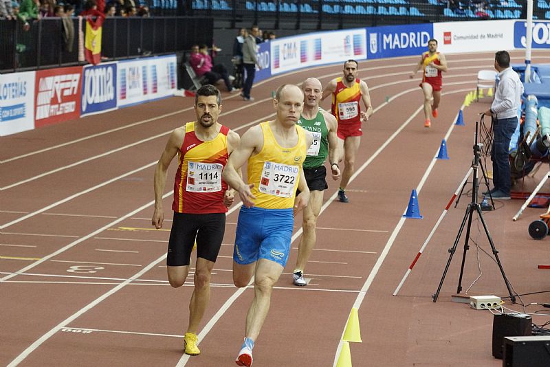
EMACI 2018 400m M40 first round (54.41).
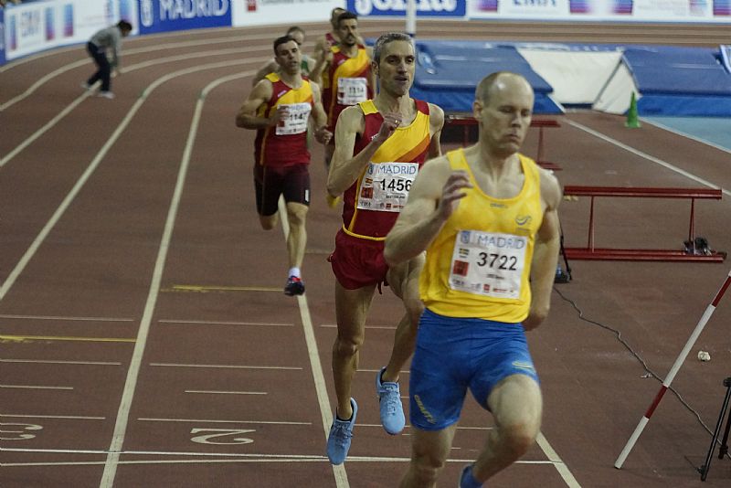
EMACI 2018 400m M40 semifinal (51.96).
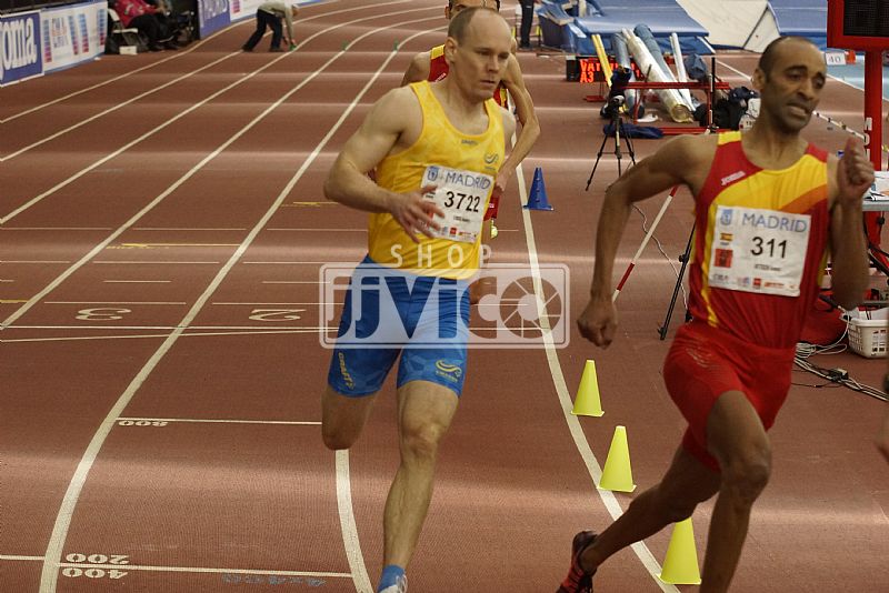
EMACI 2018 400m M40 final (52.37).
To build a model, let \(t_1\) be the split for the first 200m and let \(t_2 = f(t_1)\) be the split for the second 200m. Then the final time is \(T = t_1 + t_2 = t_1 + f(t_1)\). We also let \(t_0\) denote the fastest (not optimal) split which is identical to the 200m PR.
We now set out to determine \(f\) and subsequently find the optimal 400m time \(T^{\star} = \mathrm{min}\,T(t)\) and optimal split \(t_1^{\star} = \mathrm{arg\,min}\,T(t)\).
As per the discussion above, we make the following assumptions:
- (A1) \(f(t_0) = \infty\)
- (A2) \(f(\infty) = t_0 – 0.5\)
Assumption (A1) says that if the first 200m is run flat out, then the second 200m will be infinitely slow.
Assumption (A2) says that if one walks the first 180m, and then accelerates up to the 200m mark, then the split for the second 200m will be 0.5s better than the 200m PR as a result of the flying start. [The value of 0.5s does not have a great influence on the result and could be replaced by some other reasonable number like 1.0s.]
A simple model for \(f\) that satisfies both (A1) and (A2) is
\( f(t) = C\,(t-t_0)^{-\alpha} + t_0 – 0.5 \)where \(C, \alpha \geq 0\) are constants to be determined.
With \(t_2 = f(t_1)\), it follows that
\( \log(t_2 – t_0 + 0.5) = \log C – \alpha \log (t_1 – t_0) \)and so \(C\) and \(\alpha\) can be determined by linear regression; that is, by fitting a first degree polynomial \(y = kx + m\) to the data points of the table above with
\(\begin{array}{rcl}
x &=& \log(t_1 – t_0), \\
y &=& \log(t_2 – t_0 + 0.5).
\end{array}
\)
We may then find the parameters \(C\) and \(\alpha\) by \(C = \exp(m)\) and \(\alpha = -k\).
This is easily done using polyfit in Python (or MATLAB), see code below, and the result is \(C = 5.07\) and \(\alpha = 0.082\). The model together with the data points is shown in the figures below.
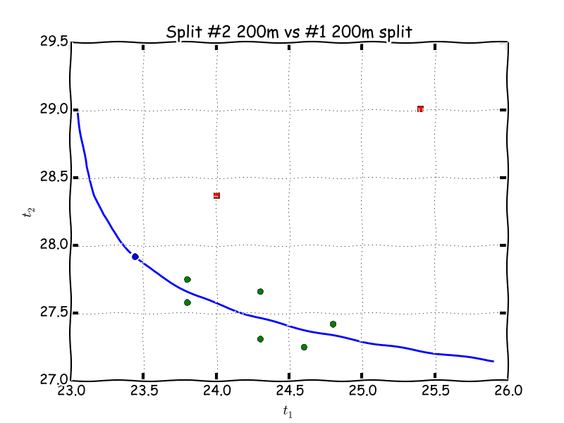
Second 200m split as function of first 200m split. Outliers are marked in red.
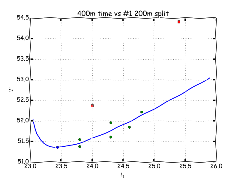
Final 400m time as function of first 200m split. Outliers are marked in red.
To determine the optimum, we note that \(T(t) = t + f(t) = t + C(t – t_0)^{-\alpha} + t_0 – 0.5\) and thus
\(T’(t) = 1 – C\alpha\,(t – t_0)^{-\alpha-1}\).
Solving for the critical point \(t_1^{\star} = \mathrm{arg\,min}\, T(t)\), we set \(T'(t_1^{\star}) = 0\) and find that
\(t_1^{\star} = t_0 + (C\alpha)^{\frac{1}{\alpha+1}} \approx 23.44\).
The prediction of the model is that the optimal 400m time is 51.36 with splits 23.44 / 27.92. This is surprisingly and interestingly close to my PR = SB = 51.38!
This indicates that I have likely done a good job of maxing out my capacity on the 400m this season, and to improve further I need to get faster (decrease \(t_0\)) and improve my endurance (decrease \(C\)).
As a final remark, it is interesting to note that at \(t = 23.8\), we have \(f'(t)\approx -0.5\), which tells us that by running the first lap 0.2s faster, I loose 0.1s on the first lap, but the net result is gaining 0.1s for the total time.
For reference I have included the Python code if anyone wants to try this at home.
# Analysis of 400m indoor 2018
# Anders Logg 2018-03-24
#
# Model: t2 = f(t1) where
#
#   f(t) = C / (t - t0)^p + t0 - 0.5
#.    t0 = 200m PR (from blocks)
#
# Note: f(t0)  = inf      (maxing out first 200m ==> failing to finish)
# Note: f(inf) = t0 - 0.5 (extremely slow first 200m ==> max second 200m)

# XKCD style plotting
from pylab import *
xkcd()

# Data
t0 = 23.0
t1 = array([24.8,  24.6,  23.8,  24.3,  23.8,  25.4,  24.3,  24.0])
T  = array([52.22, 51.85, 51.55, 51.61, 51.38, 54.41, 51.96, 52.37])
O  = [5, 7] # outliers

# Sort inliers/outliers
I = [i for i in range(len(t1)) if not i in O]
t1_i = t1[I]
t1_o = t1[O]
T_i = T[I]
T_o = T[O]

# Fit model
t2_i = T_i - t1_i
t2_o = T_o - t1_o
p, logC = polyfit(-log(t1_i - t0), log(t2_i - t0 + 0.5), 1)
C = exp(logC)
t = linspace(min(t1) - 0.75, max(t1) + 0.5)
f = C / (t - t0)**p + t0 - 0.5
print "C =", C
print "p =", p

# Compute derivative at t = 23.8
print "Derivative at t = 23.8: ", -C*p*(23.8 - t0)**(-p - 1)

# Compute optimum
t1_s = t0 + (C*p)**(1.0 / (p + 1))
t2_s = C / (t1_s - t0)**p + t0 - 0.5
T_s = t1_s + t2_s
print "Optimal split: %.2f / %.2f" % (t1_s, t2_s)
print "Optimal 400m:  %.2f" % T_s

# Plot
figure()
plot(t1_i, t2_i, 'og')
plot(t1_o, t2_o, 'sr')
plot(t, f, '-b')
plot(t1_s, t2_s, 'ob')
xlabel('$t_1$')
ylabel('$t_2$')
grid(True, lw=0.5)
title('Split #2 200m vs #1 200m split')
savefig('optimal400m_1.png')

figure()
plot(t1_i, T_i, 'og')
plot(t1_o, T_o, 'sr')
plot(t, t + f, '-b')
plot(t1_s, T_s, 'ob')
xlabel('$t_1$')
ylabel('$T$')
grid(True, lw=0.5)
title('400m time vs #1 200m split')
savefig('optimal400m_2.png')

show()