Systems of chemical reactions in FEniCS

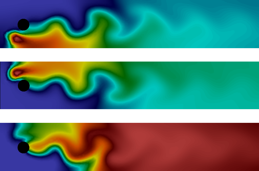
Here’s a sample from the upcoming FEniCS Tutorial that I’m currently working on with Hans Petter Langtangen. As a simple demonstration of how complex problems can be solved with a minimal amount of code in FEniCS, we simulate a system of chemical reactions taking place in a channel with the flow governed by the incompressible Navier-Stokes equations. The reaction itself is modeled as a first-order reaction using the standard advection-diffusion-reaction equation:

For the velocity field, we use a previously computed solution of the incompressible Navier-Stokes equations which we can read/write using a FEniCS `TimeSeries`. The variational problem for the equations themselves are easily implemented in FEniCS:

The solution is a quite beautiful wavelike pattern as illustrated in the following clip which plots the concentrations of the three species.

The complete code for the above simulation looks as follows.

from fenics import *

T = 5.0            # final time
num_steps = 500    # number of time steps
dt = T / num_steps # time step size
eps = 0.01         # diffusion coefficient
K = 10.0           # reaction rate
theta = 1.0        # implicitness parameter for time-stepping

# Read mesh from file
mesh = Mesh('channel.xml.gz')

# Define function space for velocity
W = VectorFunctionSpace(mesh, 'P', 2)

# Define function space for system
P1 = FiniteElement('P', 'triangle', 1)
element = MixedElement([P1, P1, P1])
V = FunctionSpace(mesh, element)

# Define test functions
v_1, v_2, v_3 = TestFunctions(V)

# Define functions for velocity and concentrations
w = Function(W)
u = Function(V)
u_p = Function(V)

# Split system functions to access components
u_1, u_2, u_3 = split(u)
u_p1, u_p2, u_p3 = split(u_p)

# Define source terms
f_1 = Expression('pow(x[0]-0.1, 2) + pow(x[1]-0.1, 2) < 0.05*0.05 ? 0.1 : 0',
                 degree=1)
f_2 = Expression('pow(x[0]-0.1, 2) + pow(x[1]-0.3, 2) < 0.05*0.05 ? 0.1 : 0',
                 degree=1)
f_3 = Constant(0)

# Define expressions used in variational forms
U_1 = (1 - Constant(theta))*u_p1 + Constant(theta)*u_1
U_2 = (1 - Constant(theta))*u_p2 + Constant(theta)*u_2
U_3 = (1 - Constant(theta))*u_p3 + Constant(theta)*u_3
k = Constant(dt)
K = Constant(K)
eps = Constant(eps)

# Define variational problem
F = ((u_1 - u_p1) / k)*v_1*dx + dot(w, grad(U_1))*v_1*dx \
  + eps*dot(grad(U_1), grad(v_1))*dx + K*U_1*U_2*v_1*dx  \
  + ((u_2 - u_p2) / k)*v_2*dx + dot(w, grad(U_2))*v_2*dx \
  + eps*dot(grad(U_2), grad(v_2))*dx + K*U_1*U_2*v_2*dx  \
  + ((u_3 - u_p3) / k)*v_3*dx + dot(w, grad(U_3))*v_3*dx \
  + eps*dot(grad(U_3), grad(v_3))*dx - K*U_1*U_2*v_3*dx + K*U_3*v_3*dx \
  - f_1*v_1*dx - f_2*v_2*dx - f_3*v_3*dx

# Create time series for reading velocity data
timeseries_w = TimeSeries(mpi_comm_world(), 'ns/velocity')

# Create VTK files for visualization output
vtkfile_u_1 = File('reaction_system/u_1.pvd')
vtkfile_u_2 = File('reaction_system/u_2.pvd')
vtkfile_u_3 = File('reaction_system/u_3.pvd')

# Create progress bar
progress = Progress('Time-stepping')
set_log_level(PROGRESS)

# Time-stepping
t = 0
for n in xrange(num_steps):

    # Update current time
    t += dt

    # Read velocity from file
    timeseries_w.retrieve(w.vector(), t - (1.0 - theta)*dt)

    # Solve variational problem for time step
    solve(F == 0, u)

    # Plot solution
    _u_1, _u_2, _u_3 = u.split(deepcopy=True)
    plot(_u_1, title='u_1', key='u_1')
    plot(_u_2, title='u_2', key='u_2')
    plot(_u_3, title='u_3', key='u_3')

    # Save solution to file (VTK)
    vtkfile_u_1 << _u_1
    vtkfile_u_2 << _u_2
    vtkfile_u_3 << _u_3

    # Update previous solution
    u_p.assign(u)

    # Update progress bar
    progress.update(t / T)

# Hold plot
interactive()